Finally, frontpage! Show HN: https://sunlight.live - A visual map of sunlight on earth.
This blogpost was written on 2019-07-03, and all data referenced are up to this date. The post itself might be published on a later date.
It feels so good showing other people your work. You can gauge reactions, get useful feedback when people give kudos for working with X or that you’re dumb for doing Y (especially the latter). The excitement is multiplied when the $thing you built can actually help people in their daily life, or when you put new skills to the test, in the real world.
Well, this is not one of these grandiose success stories, but just a little “Show HN:” submission of a project I’d build a couple of weekends ago.
The project is just a silly live-updating pixel map of sunlight on earth, showing the sun’s terminator, but somehow got on the frontpage with 74 points, reached some 18k unique visitors, 25+ GitHub stars, made me feel warm and fuzzy, and led me to learn about new things.
Needless to say, I felt giddy for this weekend idea. This post will detail both what happened during the HN “spike” as well as some takeaways and lessons learnt from actually building it.

Performance and metrics.
https://sunlight.live is hosted on a $5/mo Digital Ocean Droplet, with the following specs
| Memory | vCPUs | SSD Disk | Transfer | Price |
|---|---|---|---|---|
| 1 GB | 1 vCPU | 25 GB | 1 TB | $5/mo or $0.007/hr |
There’s no fancy infrastructure here, as I just wanted to re-learn some astronomy; I’m dealing with enough DevOps stuff day in-day out.
It’s probably the cheapest, most basic VPS available out there. The backend is a nearly-default Apache, set up on Ubuntu. Most of the deployment effort (and I mean almost 10 minutes of my time) went towards the Let’s Encrypt SSL certificate.
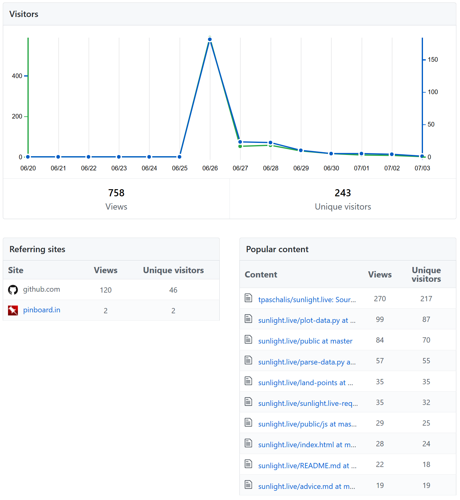
In short, this default setup was able to serve more than 410k requests and 18.5k unique visitors over these past week, (css, images, javascript and all) peaking at 64k requests per hour - 24 requests per second, pretty easily. They’re not big numbers, but at the level that a small website would start experiencing issues.
I have a dislike for pages with unnecessary third-party requests, so everything, from fonts, favicons, to javascript and images are served from this VPS, and nothing happens on the client side.
I’m also skeptical towards analytics solutions due to user privacy concerns, and avoid using them unless there’s a serious reason. So there’s no tracking and no metrics other than the Apache’s daily access.log files.
The source of these stats :
$ mkdir -p blogpost/access blogpost/error
$ sudo su -
# cd /var/log/apache2
# cp -p error.log* /home/user/blogpost/error/
# cp -p access.log* /home/user/blogpost/access/
# chown -R user:user /home/user/blogpost/
# ^D

$ echo "logrotate keeps logs from the past 14 days - /etc/logrotate.d/apache2"
$ echo "In our case we have logs between 20 June - 03 July"
$ mkdir raw
$ cp -p access/* error/* raw/
# Finally, we can start getting some stats
$ gunzip *.gz

# Total requests served
$ cat access.log* | wc -l
413223

# Number of unique IPs in requests
$ cat access.log* | awk '{print $1}' | sort -u | wc -l
18557

# Number of requests in root document
$ grep "GET / HTTP/1.1" access.log*| wc -l
24569

# Number of unique referrers.
$ cat access.log* | awk '{print $11}' | awk -F'/' '{ print $3}' | sort -u | wc -l
189

# List of requests per day
$ cat access.log* | awk '{print $4}' | cut -d: -f1 | uniq -c
# or if want to aggregate
$ cat access.log* | awk '{print $4}' | cut -d: -f1 | uniq -c | awk '{ a[$2]+=$1 } END { for(i in a) print a[i],i}' | sort -k1 -n


# List of requests per hour, for 26th of June (day I posted it on HN)
$ grep "26/Jun" access.log* | cut -d[ -f2 | cut -d] -f1 | awk -F: '{print $2":00"}' | sort -n | uniq -c
...
  49315 14:00
  64424 15:00
  38534 16:00
...


# List of hits per minute
$ grep "26/Jun" example.com | cut -d[ -f2 | cut -d] -f1 | awk -F: '{print $2":"$3}' | sort -nk1 -nk2 | uniq -c | awk '{ if ($1 > 10) print $0}'
...
   1308 14:49
   1321 15:27
   1328 15:20
   1333 15:12
   1361 15:22
   1435 15:13
   1464 15:25
What is the sun’s terminator?
The solar terminator is the imaginary line that “divides” the daylit side and the dark, night side of a planetary body.
Wikipedia states : “A terminator is defined as the locus of points on a planet or moon where the line through its parent star is tangent. An observer on the terminator of such an orbiting body with an atmosphere would experience twilight due to light scattering by particles in the gaseous layer”. I hope my explanation was a bit clearer :P You can see the sun’s terminator, as the ISS passes over Africa and the Middle East, in this seriously awesome video.
On a high-level, (just so you can impress your friends during the next trivia party):
This line, is a circle on the earth’s circumference, and passes through any point on Earth twice a day; at sunrise and sunset (except for the poles). The path of the terminator varies by time of day due to the earth’s rotation around its axis, but the shape of the curve also changes with the seasons due to the earth’s orbit around the sun. During solstice, the terminator line is at its greatest angle with respect to the axis of the Earth, which is approximately 23.5 degrees.
While one would think that each half of earth is covered in either light or darkness, the bending of the sunlight and the atmosphere scattering results in the sunlit surface being larger than the surface covered by darkness.
The terminator moves at about 1’688 kilometers per hour; while this is extremely fast, some jet fighters can overtake the maximum speed of the terminator at the equator! This means that theoretically, a plane could takeoff somewhere where the sun is rising, speed through, and land somewhere it’s still dark.
HackerNews users (sciurus, teraflop and more) pointed out that such illustrations are often found in ham radio websites, since skywave propagation between two points can vary based on the amount of sunlight. Some amateur radio operators can take advantage of the conditions of the ionosphere along the terminator, to send and receive messages at higher frequencies and much larger distances. Wikipedia also states that “Under good conditions, radio waves can travel along the terminator to antipodal points (diametrically opposite points of the earth!!)”. Just HOW cool is that.
Finally, the examination of the terminator can yield information about the surface of a planetary body. A fuzzier terminator might signify the existence of an atmosphere.
Some low-earth orbit (LEO) satellites take advantage of the fact that when flying in certain orbits near the terminator, the sun is always visible, therefore they can keep charging their solar cells at all times. These types of orbits are called ‘dawn-dusk’ orbits, and can prolong the lifecycle of a LEO satellite.
Boring math stuff :
While the math involved is simple additions and multiplications, calculating the sun’s position involves multiple steps, and understanding some concepts such as the ecliptic coordinate system, the sun’s declination, hour angles etc.
I was lucky to have some good teachers in my Physics years, so tracing back to my textbooks was easier than I expected. There’s an awesome course in Greek about celestial mechanics, available by the University of Crete as a MOOC.
Wikipedia, as always, has some excellent information, along with examples to get one started.
And while all this can be confusing, I stumbled upon an awesome website by Dr Louis Strous. It’s an old-school, information-dense website, with questions, exercises, and their answers about celestial mechanics, astronomical formulas, and general cosmology. The bibliography page is a nice collection of resources as well.
His website provides a straightforward way to trace the path of the terminator for any time and day, throughout the year. The result is accurate up to 1 degree, which is good enough for our pixel map.
In short :
- Calculate the sun’s mean anomaly, M
- Calculate an approximation of the sun’s ecliptic longitude, lambda - λ
- Calculate the sun’s declination, delta - δ
- Then, at t hours UTC, the sun is on its zenith (fancy word for ‘straight up’), from :
- a location of latitude b, equal to the declination δ and
- a longitude equal to l = 180 - 15 * t degrees.
- If ψ is the distance in degrees from one of its intersections with the equator, then the eastern Longitude L and the northern Latitude B, at the point ψ can be found as
- B = arcsin(cos(b)•sin(ψ))
- x = -cos(l)sin(b)sin(ψ) - sin(l)cos(ψ)
- y = -sin(l)sin(b)sin(ψ) + cos(l)cos(ψ)
- L = arctan(y, x)
- That’s all! L and B are the points of the terminator, so run ψ from 0 to 360 degrees!
A solid line?
A feature proposed by many people was to have a gradient instead of a solid terminator line, as there’s not really a hard cutoff between what we define as ‘day’ or ‘night’.
When using Zenith for calculations, there are various definitions of ‘twilight’, such as the Civil Twilight, the Nautical twilight, the Astronomical twilight. timeanddate.com uses this approach for their terminator map and provide the info with some nice shades.
I used the most popular definition, the “civil” twilight; it’s minutes after the sun has set, and the sky is pretty at that time ^^
Modifying the code to produce these shades or a continuous gradient should not be very difficult, after all we’re almost done computing the necessary astronomical features. It’s just a matter of providing the correct shades to part of our scatter plot. I might indeed do it at some point, but I’m currently liking the two-color, minimal scheme, and I don’t know how the gradient would translate on the dark background.
Matplotlib
I really like matplotlib. After working with the pandas/numpy/pyplot/matplotlib gang for some time, I feel that the main problems people face when plotting can be traced back to either them not reading the documentation, or getting confused because there’s multiple ways to achieve the same result. Especially since many things can be accomplished both using a procedural syntax and a method, eg this. StackOverflow has an abundance of answers, and rushing to copy/paste things will only increase confusion.
You have to sit down, decide what you want to draw, how it translates to matplotlib objects, define your graphs, and get the data! Or else, you’re going to end up like :
What’s a canvas? Is it the same as a figure? How about adding a subplot, where should I define it? Where do you want your separate axes? Are they defined for each figure, or for each canvas? No I don’t mean the matplotlib figure object, I mean the figure that we’re printing for our paper. ARGH. Labels and Titles for each sub-graph (how are they called in matplotlib again)? Darn, I’m using MS Paint after all, deadline is tonight at 9…
Here’s the simple case used in the repo. I’m not an expert by any means, and I’m just now starting to wrap my head around how all these things get tied together to build more complex and beautiful graphs, but I’d say the result is pretty clean, easy to understand and modify. My rule of thumb is to just start with the figure, define and name your objects procedurally, and then just use methods consistently.
import matplotlib
import matplotlib.pyplot as plt
import numpy as np

...

matplotlib.use('Agg')		 	# Use a backend that doesn't display to the user, so the code can run in the background batch.
fig = plt.figure()
fig.set_size_inches(24,12)		# World map will be drawn on a (20,10) inch grid, w/ (2,1) margin on each side
fig.set_dpi(300)			# Setting the DPI too low results in render artifacts between dots
fig.set_tight_layout(True)

canvas = fig.add_subplot(111)
canvas.set_xlim(left=-200, right=200)
canvas.set_ylim(bottom=-110,top=110)
canvas.set_aspect('equal')
canvas.set_facecolor((0.8, 0.8, 0.8))
canvas.set_axis_off()

...

# Sort the terminator points in pairs
xT, yT = (list(t) for t in zip(*sorted(zip(xT, yT))))
terminator = canvas.plot(xT, yT, c="red")

# Draw the pixel world map. Marker size is related to their area
# We select a marker size, so that our plot can acommodate 360*180 points
# https://stackoverflow.com/questions/14827650/pyplot-scatter-plot-marker-size
x, y = [], []
...
canvas.scatter(x, y, s=2)

# Interpolate the points of the terminator for each degree.
# This way we can draw the 'daylight' points in a different color

x1, y1 = [], []
...
canvas.scatter(x1, y1, c = (0.8, 0.8, 0.8),  s=2)

fig.savefig('public/images/output_term.png', dpi='figure', format="png", transparent=True)
Map Data
For this project needed world-wide mapping data. There are different ways to achieve this, but most straightforward way I found was to use the wonderful Natural Earth dataset. It’s built by a collaboration of volunteers and is supported by the NACIS (North American Cartographic Information Society). The Terms of Use are very generous, citing that “All versions of Natural Earth raster + vector map data found on this website are in the public domain. You may use the maps in any manner … The primary authors, … invite you to use them for personal, educational, and commercial purposes”.
So I’d definitely suggest looking into them for your next cartography project and/or support their cause!
The data comes in the “ESRI shapefile format”, which is the de facto(?) standard for vector geodata. Geopandas is an excellent Python framework, that allows to use your pandas knowledge in mapping projects, as it can handle .shp files.
The resulting Geopandas object is a geopandas.geodataframe.GeoDataFrame which works like pd.dataframe with columns ‘featureclass’, ‘scalerank’, ‘min_zoom’, and ‘geometry’.
  featurecla  scalerank  min_zoom                                           geometry
0       Land          1       1.0  POLYGON ((-59.57209469261153 -80.0401787250963...
1       Land          1       1.0  POLYGON ((-159.2081835601977 -79.4970594217087..
Here’s the simple code I used to gather all the points on earth that fall on land, in a 1 degree resolution.
import os
import geopandas as gpd
import matplotlib.pyplot as plt
from shapely.geometry import Point, Polygon

#gdf = gpd.read_file('ne_50m_land/ne_50m_land.shp')
print("gdf :", type(gdf))       # The object is a <class 'geopandas.geodataframe.GeoDataFrame'>

polygons = gdf["geometry"]      # Keep the polygons column that define the land data.
print(polygons.shape)

landX = []
landY = []
for i in range(-180, 180, 1):   # For each point in our pixel map, check if is Point(i,j).within any "Polygon"
    print(i)
    for j in range(-90, 90, 1):
        for poly in polygons:
            if Point(i, j).within(poly):
                landX.append(i)
                landY.append(j)

with open("land-points-shapefile", "w") as f:
    if len(landX) != len(landY):
        os.Exit(1)
    for i in range(len(landX)):
        f.write(str(landX[i])+","+str(landY[i])+"\n")

gdf.plot()
plt.show()
Design and Optimization
I’m probably one of the worst designers out there; my modus operandi in developing websites is to frantically copy/paste CSS rules from Stack Overflow and hitting the refresh button. God forbit I want to move an element from one part of the page to another, it’s a recipe for disaster!
So naturally, I started by shamelessly stealing copying borrowing ideas off other websites and templates, to get a minimalistic, clean starting point. The initial size of the template page was around 2.5MB.
Right now, a fresh start of the website weighs 487 kB. The displayed image takes the cake with 404kb, while everything else, from CSS, JS, icons comes back at 83 kB. It’s not great, but I’m just content that the website is not bloated to the point that it takes up more space than “Crime and Punishment”.
I didn’t do anything groundbreaking other than remove all non-essential CSS (oh God, so much crap CSS), decide on a minimal set of JS files so that the website works fine on mobile, and cut out silly fonts and icon files. For example, initially I had imported the entirety of FontAwesome icons, in various formats. One step was to use Fontello and serve only the icons I need and in just two formats .svg and .woff.
The process was done manually using Firefox’s console, and is not something I’d like to spend more time on, so if anyone has any adequate automated solution, please reach out!
Using these simple steps, the original template size was reduced in about 1/30 of the initial size. There’s still much room to trim things down, but I got to a point where some of my efforts were either breaking down the website’s mobile appearance, or led to wrong scaling on different orientations, so I called it a day.
The main things I have to try right now are
- to minimize the image size and/or serve different images depending on the end user resolution
- use a caching layer, other than the browser’s, if needed
- see if there’s a user benefit from me using a CDN.
What did you learn?
The internet community can be nice when they want to! I had strangers sharing ideas on how to improve the project, posting their own projects and code, raising issues, and even opening Pull Requests (ty Jacek!).
I’m still getting twitter replies and emails from people who liked and shared sunlight.live on their own blogs, so I’m extra happy they took the time to spread the word.
I’m pretty sure that a good README.md would have helped more people extract value from the repo. Things I should have added :
- Explanation of design decisions and failed tries
- Key takeaways
- Small guide on how to run your own copy/modify the code
- Small tutorial on how to write clean matplotlib code.
I will make sure to fix this, and that my next projects will have a better ‘store-front’ face.
I learned a lot about html and css, and I can say with confidence that this it not my favorite layer of the stack.
Well, until next time!